Feature Extraction – Gabor Filters

If you have read any article on texture segmentation, then you might have come across Gabor filters. Yes, they are used for other applications too, like enhancement, edge detection, document analysis etc. So, what are Gabor filters? Do they really work like a regular filter that reduces noise present in a signal?

To know what they are you have to patiently read through rest of this article.

Since this blog focuses on Computer Vision, we will consider only 2D Gabor filters. But, if you are interested in 1D Gabor filters you may find this article useful (Images are easier to visualize than 1D signals.)

What makes Gabor filters special? As you know, when it comes to vision systems, human visual system remains undefeated. Gabor filters kind of mimics the human visual system. Thus a set (yes; a set. We usually use more than one Gabor filter) of Gabor filters can be used to determine or preserve the orientation or scale of edges in an image

Since we know that Gabor filters are amazing, let’s touch upon the mathematical side of these filters. Gabor filter consists of two components,

• Complex sinusoid (s(x,y)), known as carrier.
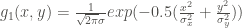
• Gaussian function,(g(x,y)) known as envelope.

The complex sinusoid is defined as,

Where, is the orientation of the complex sinusoid, F is the magnitude of the sinusoid and P denotes phase and the Gaussian function is defined as:

In order to rotate the Gaussian function in the direction of the complex sinusoid, we have to modify the Gaussian function as:

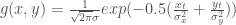
where,

Thus, the 2D Gabor filter is given by,

Now, let’s visualize the above equations. Start MATLAB and run the following code:

%Defining parameters
img_size = 90;          %Size of the image
theta = 90;             %Orientation of the signal
F = 1/20;               %Magnitude of the signal
phase = 0;              %Phase of the signal

%Generating X and Y coordinates
[y x]=meshgrid(-round(img_size/2):round(img_size/2),round(img_size/2):-1:round(-img_size/2));
%Carrier signal
carrier_signal = real(exp(1i*(2*pi*F*(x*cosd(theta) + y*sind(theta))+phase)));
%Displaying the signal
imshow(carrier_signal,[]);
title('Carrier Signal');

I ran the above code for theta = {0,90,45,65} degrees. The result is shown in Fig 1

Figure 1: Carrier signal for different values of theta

Now to visualize the Gaussian envelope, run the following code

%Defining parameters</pre>
<pre>img_size = 90;          %Size of the image
theta = 0;              %Orientation of the signal
sigma_x = 5;            %Standard deviation along x-axis
sigma_y = 20;           %Standard deviation along y-axis

%Generating X and Y coordinates
[y x]=meshgrid(-round(img_size/2):round(img_size/2),round(img_size/2):-1:round(-img_size/2));
%Carrier signal
x_t = x*cosd(theta) + y*sind(theta);
y_t = -x*sind(theta) + y*cosd(theta);
gaussian_env = exp(-0.5*(x_t.^2./sigma_x^2 + y_t.^2./sigma_y^2));
%Displaying the signal
imshow(gaussian_env,[]);
title('Gaussian envelope');

The result of the above code is shown in Fig 2

Figure 2: Gaussian envelope for different values of theta

When we multiply the carrier signal and the gaussian envelope, the obtain Gabor filters.

%Multiply gaussian envelope and carrier signal
Gabor_kernel = gaussian_env.*carrier_signal;

%Display the image
imshow(Gabor_kernel,[]);
title('Gabor kernel');

The Gabor kernel for different values of theta is shown in Fig 3.

Figure 3: Gabor kernels for different values of theta

In the image shown in Fig 4, we have lines oriented at 0, 45, 90 and 135 degrees.These Gabor kernels are used to find edges oriented in any given direction i.e. if we convolve an image with a Gabor kernel with theta = 45 deg,we will obtain strong response if there are edges oriented at 45 deg.

Figure 4: Test image

Figure 5: Result of applying gabor kernels on the test image

It is evident from Fig 5, that in the convolved images edges oriented in the direction of the Gabor kernel has produced a strong response. This can be used to detect lines in any orientation or analyse texture. How? Say if you wanted to find whether any line inclined at 45 degrees in Fig 4. When you multiply the image with Gabor kernel with theta = 45 deg, you will get a high response as shown in Fig 5. This is used to detected line inclined at 45 deg.When we convolve the above image with Gabor kernels with theta = (0, 45, 90, 135) we obtain responses as shown below:

Seems like a simple concept – gabor filters, but it is widely used in computer vision to detect textures. I’ll soon write a post on texture classification using gabor filters.
C++ code

Have a great day.. 🙂

(If you have any questions or find any mistakes please leave a comment below. You will be properly acknowledged for finding errors)

Outlier elimination – Tukey’s method

I was working on a classification problem using machine learning and while analyzing the training data, I noticed that there were few data points which didn’t fit the distribution. These data points were making the gaussian distribution not gaussian.

To improve the accuracy of the classifier, I needed to eliminate them. For that purpose, I used Tukey’s method. It uses interquartile range to find/eliminate outliers.

What is a Quartile and how to find Interquartile range?

If we divide the data into 4 sections, each containing 25% of the data, then each section is called a Quartile. The data is sorted in an ascending order. The first 25% of the data is called 1st quartile, 25% – 50% is called the 2nd quartile, 50% – 75% is called the 3rd quartile and the last 25% is called the 4th quartile.

In Python, we can calculate quartiles as follows:

def GetQuartiles(arr):
    arr = np.sort(arr)
    mid = len(arr)/2
    if(len(arr)%2 == 0):
        Q1 = np.median(arr[:mid])
        Q3 = np.median(arr[mid:])
    else:
        Q1 = np.median(arr[:mid])
        Q3 = np.median(arr[mid+1:])
    return Q1,Q3

For the dataset shown below, the quartile are:

The distance between 3rd quartile and the 1st quartile is called Inter-Quartile Range (IQR.)

How to detect Outliers using IQR?

Anything which lies below (1st quartile – IQR) or above (3rd quartile + IQR) are considered as outliers. But, you can multiply a small bias with IQR to include/exclude more data points.

def EliminateOutliers(arr, bias = 1):
     q1,q3 = GetQuartiles(arr)
     iqr = q3 - q1
     lowerLimit = q1 - bias*iqr
     upperLimit = q3 + bias*iqr
     return filter(lambda x: (x > lowerLimit and x < upperLimit),arr)

For bias = 1, the outliers are highlighted below.

This is a simple method to eliminate outliers in the data and help you to train a better classifier.